Surrogate models
Overview
Fitting the data with the command profit fit is accomplished by
Gaussian process regression (GPR) surrogate models.
Currently, there are three such models implemented in proFit, which differences are explained further below:
Custom (built from scratch in proFit)
GPySurrogate (based on GPy)
SklearnGPSurrogate (based on scikit-learn)
There are also two multi-output models:
- CustomMultiOutputGP (based on the Custom surrogate)
Implements simple, independent GPs in every output dimension.
- CoregionalizedGPy (based on the GPySurrogate)
Uses the coregionalization kernel from GPy to model dependencies between outputs.
Under development:
Artificial neural network surrogate (using PyTorch)
Design
The hierarchy of implemented models is shown in the figure below. The universal
Surrogate class is the overall base class of surrogates, which functions as abstract
base class where models are registered. For experienced users, this allows implementing
fully customized surrogates, starting from importing one of the available
classes and modifying only one method, to writing new classes from scratch which
integrate in the workflow by standard methods like train, optimize, predict,
save_model, and load_model. These methods are used throughout every sub
class to ensure compatibility between surrogates, encoders, and active learning
algorithms:
trainTrains the model on a dataset. After initializing the model with a kernel function and initial hyperparameters, it can be trained on input data \(X\) and observed output data \(\mathbf{y}\) by optimizing the model’s hyperparameters, which is done by minimizing the negative log-likelihood.
optimizeFinds the optimal hyperparameters of the model to ensure consistency with observed data.
predictPredicts the output at test input points \(X_*\) by building the posterior mean and covariance using previously trained data.
save_modelSaves the model and used encoding as Python dictionary to a .hdf5 file. For the coregionalization multi-output surrogate from GPySurrogate , a .pkl file is used instead.
load_modelLoads a saved model from a .hdf5 (or .pkl) file, updates its attributes and restores the encoding.
To be able to use the surrogate in active learning, another two methods are necessary:
add_training_dataAdds \(X\) and \(\mathbf{y}\) data to the model.
add_ytrainOverwrites the placeholder \(\mathbf{y}\) data inserted during active learning with the actual data.
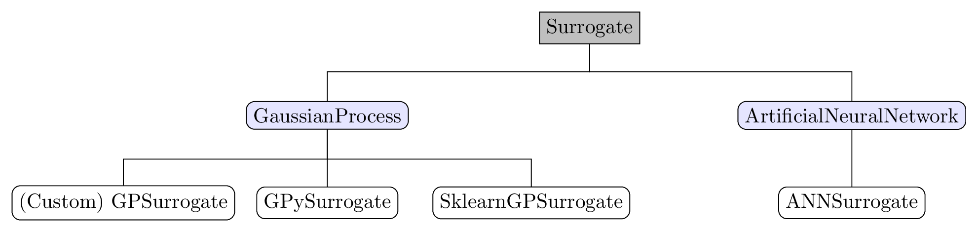
Surrogate hierarchy. Grey: base class, blue: intermediate helper class, white: user selectable classes.
Each of the above mentioned GP surrogate models has its own advantages, the most important of which for the use in proFit are displayed in the following table:
Surrogate
(Identifier)
|
Advantages
|
|---|---|
GPSurrogate
(Custom)
|
Built from scratch.
Well suited for study purpose.
Customizable kernels in Python and Fortran.
Customizable optimization (Laplace approximation,
include derivatives, etc.).
|
GPySurrogate
(GPy)
|
Large number of selectable models and kernels.
Multi-output models with coregionalization available.
Small package size.
|
SklearnGPSurrogate
(Sklearn)
|
Low level customization possible.
Good integration with other scikit-learn libraries.
|
Kernels
For the GPySurrogate and the SklearnGPSurrogate the respective kernels of their packages can be
called by their corresponding class name.
The kernels of the custom GPSurrogate are implemented by default in Python and Fortran,
where the RBF,
Matern32 and
Matern52 kernels are available as of now.
The automatic relevance detection (ARD) feature of the GPy kernels can be used for dimensionality reduction, as dimensions with large length-scales are excluded from the fit which makes the model less complex.
Encoders
Encoding of input and output data is an important topic as well, as it can make surrogate models more reliable. The most important encodings in proFit include
- Normalization
The fit is always executed on the \(n\)-dimensional \(1\)-cube with zero mean and unit variance, which usually makes the surrogate models more reliable for data with a large range. It is also planned to implement an encoder to handle heteroscedastic data.
- Exclusion
Specified dimensions of the data are neglected from the beginning which makes the fitting procedure more efficient, as less dimensions have to be considered.
- Log10
The transformation \(log(x)\) is applied which can reduce model complex- ity, as e.g. a linear model can be fitted instead of an exponential one.
- Dimensionality reduction
Transformations can be applied, e.g. principal component analysis (PCA) and Karhunen-Loeve decomposition (KL) which contribute to minimizing computational effort of fitting high dimensions. The difference between PCA and KL here is that PCA is conducted with the collocation matrix \(M=X^T \cdot X\) which is efficient if the number of samples is greater than the number of variables, while KL uses the covariance matrix \(C=X \cdot X^T\) which is efficient if the number of variables is larger than the number of samples.
By default, the following encoder pipeline is used:
Exclude
Constantinput variablesLogarithmically transform
LogUniforminput variablesNormalize all input variables
Normalize all output variables
Custom encoders can be registered to the base Encoder class, as described generally in
Custom extensions.
Examples
fit:
    surrogate: GPy
    save: model.hdf5  # Automatically becomes model_GPy.hdf5 for identification.
    fixed_sigma_n: False  # Fix noise in the beginning.
    kernel: RBF  # Also possible, e.g.: `Matern32`, `Matern52`, etc.
    hyperparameters:  # Initial hyperparameters. Inferred from training data if not given.
        length_scale: 0.1
        sigma_f: 1.0
        sigma_n: 0.01
    encoder:
        - Exclude(Constant)  # Applied on `Constant` variables.
        - Log10(LogUniform)  # Applied on `LogUniform` variables.
        - Normalization(all) # Applied on all input and output variables.
fit:
    surrogate: CoregionalizedGPy  # Use coregionalization multi-output surrogate.
    save: model_CoregionalizedGPy.pkl  # Only saving to `.pkl` is implemented for this surrogate.
    encoder:
        - Log10(input)  # Transform all input variables.
        - KarhunenLoeve(output)  # Use dimensionality reduction encoder on output.
        - Normalization(all)  # Normalize all input and output variables.
fit:
    surrogate: GPy
    load: model_1.hdf5  # Load already trained model.