Active Learning

Besides running simulations and building surrogate models afterwards, proFit provides algorithms to execute this simultaneously by active learning (AL). AL allows to reduce the necessary number of training points to reach a specific fit quality compared to sampling from a random or Halton distribution, as points can be chosen directly where most information is gained. proFit implements two algorithms by default, called SimpleAL and McmcAL. The former serves as the default active learning algorithm by which consecutive points are chosen according to some acquisition function, like minimization of the fit variance or finding the maximum of a function.

The second provided method is a Markov-Chain-Monte-Carlo (MCMC) algorithm, which is a somewhat different use case of proFit, compared to the other modes and the SimpleAL algorithm, as it makes use of already observed experimental data and a parameterized model to find the posterior distribution of these parameters, instead of fitting a non-parametric Gaussian process. It implements the additional feature of delayed acceptance, which further reduces computational effort. The MCMC algorithm is discussed separately in Markov-Chain Monte-Carlo.

In the SimpleAL algorithm a warmup method is implemented, where initial points are sampled randomly, to receive a first estimate of the surrogate model. Thereafter in the learn method, where the main loop is contained, the acquisition function finds the next best points which are injected into the run queue. The model and fit are updated and the successive next best points are searched. This workflow is shown graphically in the figure below:

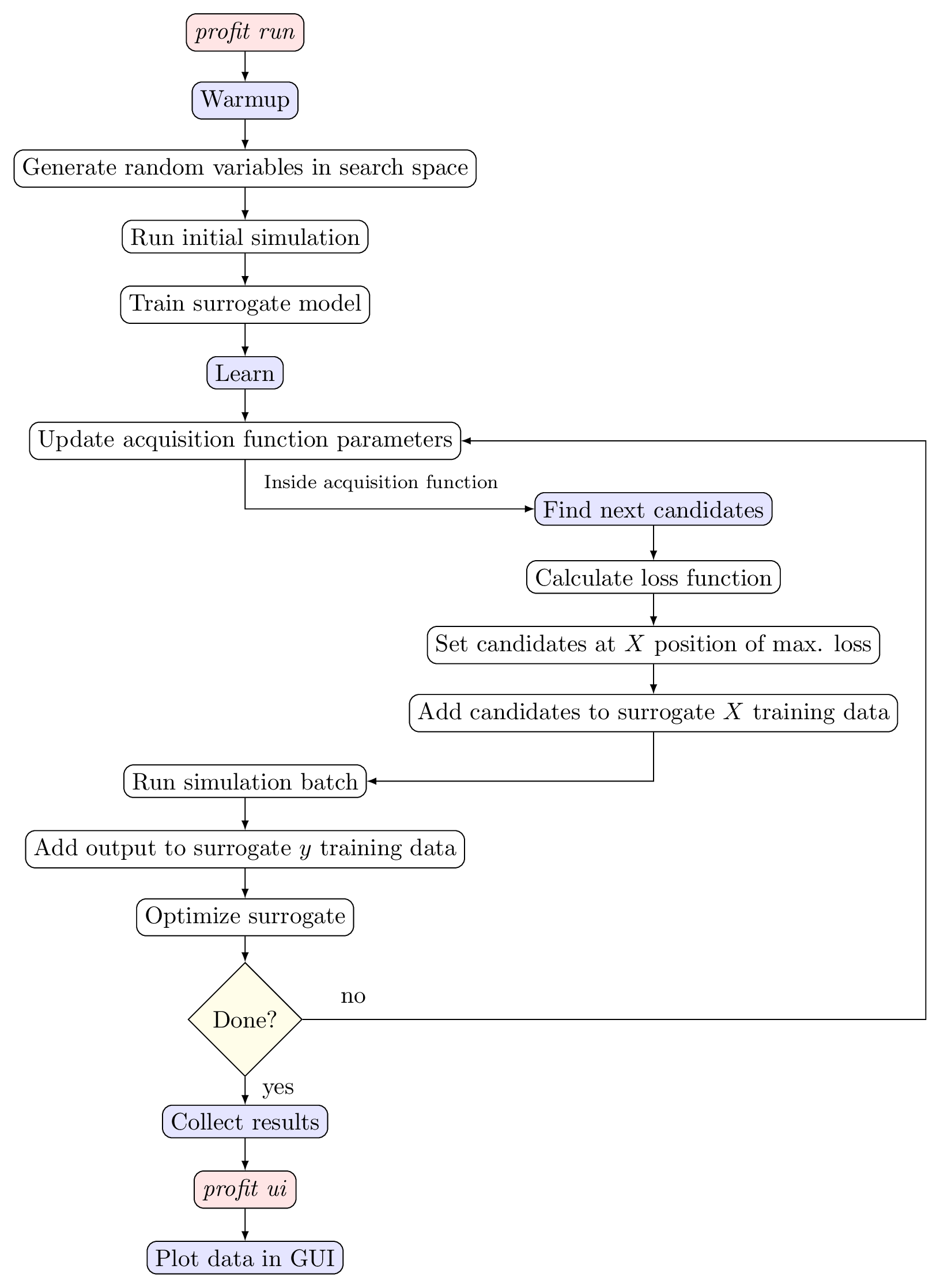
_images/al_workflow.png — Active learning workflow

proFit automatically activates AL if the user inserts an ActiveLearning variable inside the profit.yaml configuration file. The corresponding search interval is given as parameter of the variable, defaulting to \([0, 1]\). As optional parameter, the AL variable can be set to log-space, which means the search space is logarithmically transformed. This especially makes sense if the user wants to explore a large space. Multi-dimensional active learning is also possible by defining several AL variables. In this multi-dimensional case, Gibbs sampling is used, as of now. Furthermore, AL and non-AL variables can be combined to perform active learning only in certain dimensions. The distinctive parameters of the AL algorithm and acquisition functions are adjusted in the section active_learning of the config file. A special parameter to be mentioned is the batch_size, which allows to search for several points in parallel. This is especially useful, as today’s computing clusters are much better utilized if computing in parallel.

Acquisition functions

The task of an acquisition function is to find points which yield the most information according to a loss function and should be explored next by the simulation. An overview of in proFit implemented acquisition functions and a short description of their purpose is shown in the table below:

Acquisition function (Identifier)	Task
Simple exploration (simple_exploration)	Minimize fit variance. Optional `bool` parameter: `use_marginal_variance`. take into account derivative of hyperparameters (only for Custom surrogate).
Exploration with distance penalty (exploration_with_distance_penalty)	Minimize fit variance. Exponential penalization of nearby points with the `weight` parameter.
Weighted exploration (weighted_exploration)	Minimize variance. Or maximize surrogate mean. Adjustable by the `weight` parameter.
Probability of improvement (probability_of_improvement)	Find global maximum or minimum. Adjustable exploration part to avoid confinement in local extremum. (Parameter `exploration_factor`)
Expected improvement (expected_improvement)	Find global maximum or minimum. Adjustable exploration part to avoid confinement in local extremum. (Parameter `exploration_factor`)
Alternating exploration (alternating_exploration)	Alternating simple exploration and expected improvement during learning cycles. Parameters of `simple_exploration` and `expected_improvement` as well as `alternating_freq` to indicate the frequency of changing between the two acquisition functions.

Parallel active learning

With today’s supercomputers, parallel computing has become an integral part of numerical simulations. Even for expensive simulations it is thus more efficient to select several points at once instead of evaluating one point after another. For active learning this means also the search for candidates has to be parallelized to find a next best batch instead of the next best point. For the simple exploration acquisition function, this is done straightforwardly, as the predictive variance \(\mathbb{V}\) does not depend on the actual simulation output \(\mathbf{y}\):

\[\mathbb{V}[\mathbf{y}_*] = K_{**} - K_*^T (K + \sigma_n^2 I)^{-1} K_*\]

with \(K = k(X, X)\) the training kernel matrix, \(K_* = k(X_*, X)\) and \(K_{**} = k(X_*, X_*)\). \(X\) represents the training input points, \(X_*\) the prediction input points, \(\mathbf{y}_*\) the prediction output and \(I\) the identity matrix and \(\sigma_n\) the data noise.

For other acquisition functions that depend on the evaluated output \(\mathbf{y}\), approximations with the predictive fit itself, i.e. with \(\mathbf{y}_*\), have to be made.

As an example, in the expected improvement acquisition function, the exploration and exploitation parts are split, so the exploration can be fully parallelized and updated for each point in the batch. The exploitation term, on the other hand, is approximated by the mean function of the given surrogate model at the beginning, and is not updated throughout the batch.

Examples

ntrain: 50  # Points in total (AL warmup + AL learn).
variables:
    u: ActiveLearning()  # AL variable in interval [0, 1].
    v: ActiveLearning(1e-4, 1, Log)  # AL variable with log search space.
    mu: Normal(0, 0.2)  # Non-AL variable (Gaussian distributed).
    f: Output  # Scalar output.

run:
    ...  # Usual run configuration

fit:
    surrogate: GPy  # Use this surrogate during AL.

active_learning:
    nwarmup: 10  # Randomly sampled warmup points.
    batch_size: 1  # Sequential learning.
    algorithm:
        class: simple  # SimpleAL
        acquisition_function: simple_exploration  # Minimize fit variance.

...
active_learning:
    nwarmup: 4
    batch_size: 16  # Parallel learning
    algorithm:
        class: simple
        acquisition_function:
            class: alternating_exploration  # Alternate `simple_exploration` and `expected_improvement`
            exploration_factor: 0.1  # Exploration factor for expected improvement.
            find_min: True  # Find function minimum instead of maximum.
            alternating_freq: 2  # Do exploration twice, then expected improvement twice.