Markov-Chain Monte-Carlo

The Markov-Chain-Monte-Carlo algorithm (MCMC) is closely related to active learning but candidate points are sampled from a distribution and either accepted or rejected according to their posterior probability rather than actively learned. Furthermore, MCMC focuses on finding the highest posterior distribution of the parameters in place of optimizing a loss function as in active learning.

Given observed data and a simulation model with certain (physical) parameters, an MCMC simulation estimates the best posterior distribution of these parameters.

The ingredients to an MCMC algorithm are the following:

• Data

  Observed (experimental) data. Which path is given in the configuration as parameter reference_data.

• Model simulation

  Usual simulation to model the observed data with parameter vector \(\theta\).

• Sampling algorithm

  Method, how next input points to the simulation are chosen. In proFit the Metropolis-Hastings algorithm is used.

• Likelihood function

  Function to compare candidate points with already sampled points. In proFit, a Gaussian likelihood is chosen.

As the initial MCMC point starts at a random position in search space, warmup cycles are necessary to reach the desired area of high posterior probabilities. A widely used target acceptance rate of accepted versus rejected points is the well known asymptotically optimal target acceptance rate of \(0.234\). This value has to be treated with caution, as there may be significantly better suited acceptance rates for a particular problem. The target acceptance rate can be adjusted in the configuration with the parameter target_acceptance_rate. Given a specific target acceptance rate, the step size of how far in some direction in parameter space the next point is chosen, is adapted throughout the warmup cycles. After all warmup cycles are complete, the warmup points are discarded and the actual MCMC run, which yields the final posterior distribution with uncertainties for the parameters, is executed. The config parameter last_percent specifies which fraction of the main MCMC run is used for calculating the mean and variance of the posterior distribution. This lasts normally until a convergence criterion is satisfied or the maximum number of MCMC runs is reached. The log-likelihoods of each step are saved to ./log_likelihohod.txt and the parameter’s final mean and standard deviation are saved to ./mcmc_stats.txt.

A special feature of the proFit MCMC algorithm is delayed acceptance (DA), which uses a surrogate model of the loss function to estimate its expected minimum and can thus reject prospected MCMC points by the surrogate model, already before an (expensive) simulation run is started, which can reduce computation time. As of now, DA can be utilized only after the first warmup cycle. Before, points are accepted or rejected only by running the simulation. It is planned to use the SimpleAL active learning algorithm to also sample the first points intelligently. Delayed acceptance can be activated in the configuration by setting the parameter delayed_acceptance.

Results

Setting the parameter make_plot in the active_learning section plots the MCMC results for each warmup cycle and the main MCMC loop.

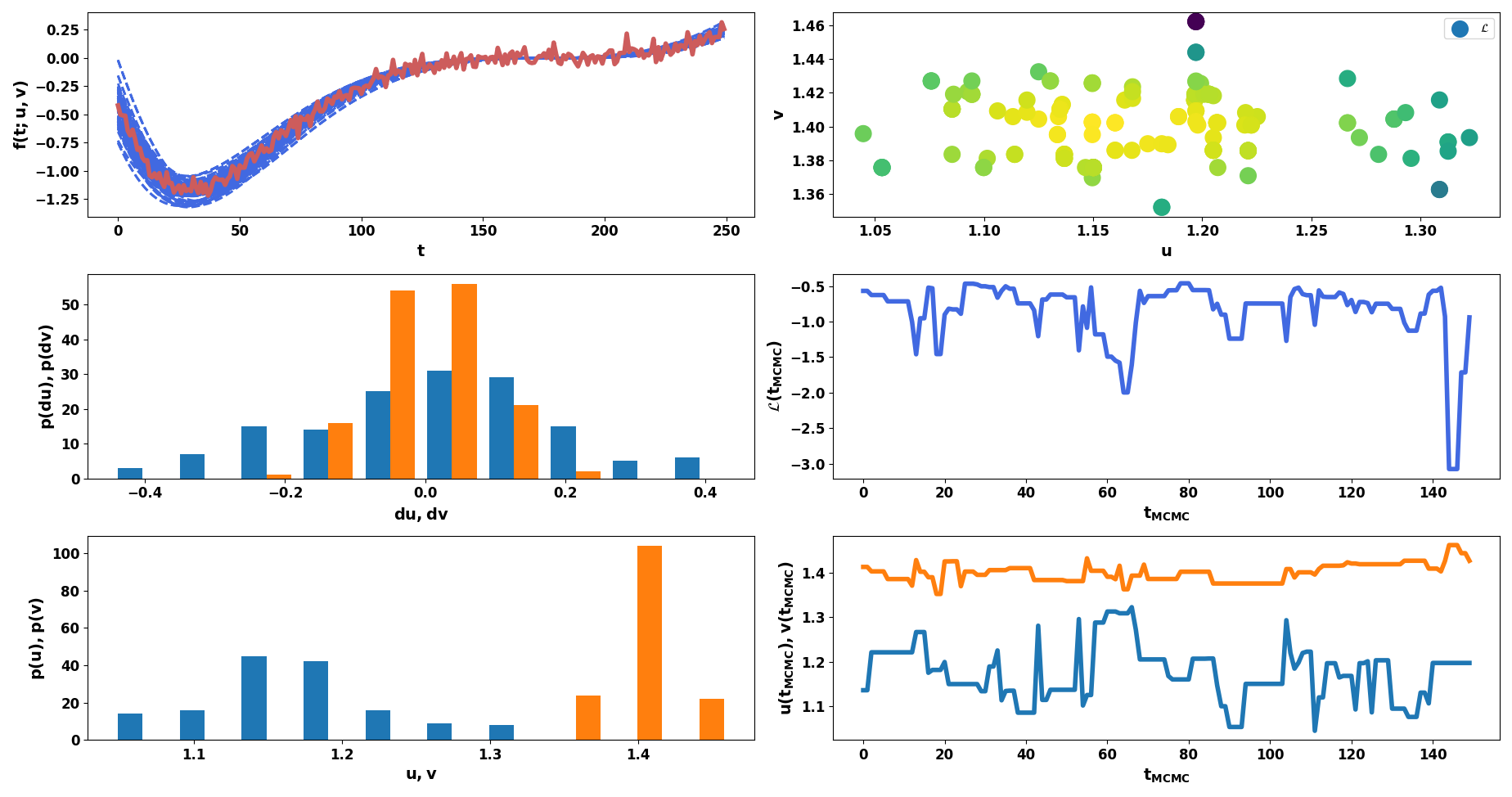
Example MCMC results. Upper left: Experimental data (red) and simulation evaluations with two parameters (blue). Middle left: Distribution of step sizes for each MCMC step per parameter. Lower left: Posterior distribution of parameter values. Upper right: Likelihood for each observed sample. Middle right: Likelihood as function of MCMC steps. Lower right: Parameter values as function of MCMC steps.

Examples

ntrain: 1000  # Total number of training points.
...
active_learning:
    nwarmup: 50  # Number of warmup points per cycle
    algorithm:
        class: mcmc
        reference_data: ./experimental_data.txt
        warmup_cycles: 5
        target_acceptance_rate: 0.35
        sigma_n: 0.05  # Estimated data noise (standard deviation)
        initial_points: [0.5, 1]  # Starting points for each dimension. If None, randomly chosen in search space.
        last_percent: 0.25  # Last points used to calculate mean and variance of posterior.
        save: ./mcmc_model.hdf5  # Save MCMC model path.
        delayed_acceptance: True  # Use delayed acceptance with surrogate specified in `fit` configuration.