Example: Surrogates
Showcases the API usage of GP and LinReg Surrogates in 1D and 2D
Note: these examples use mostly the default values. Better results can be achieved if hyperparameters are set manually to known values (e.g. if the uncertainty is known).
[1]:
# import libraries
import numpy as np
import matplotlib.pyplot as plt

rng = np.random.default_rng()
[2]:
# import the Surrogate
from profit.sur import Surrogate

# ensure GP and LinReg Surrogates are available
import profit.sur.gp
import profit.sur.linreg
[3]:
# available surrogates:
Surrogate.labels
[3]:
{'GPy': profit.sur.gp.gpy_surrogate.GPySurrogate,
 'CoregionalizedGPy': profit.sur.gp.gpy_surrogate.CoregionalizedGPySurrogate,
 'Custom': profit.sur.gp.custom_surrogate.GPSurrogate,
 'CustomMultiOutputGP': profit.sur.gp.custom_surrogate.MultiOutputGPSurrogate,
 'Sklearn': profit.sur.gp.sklearn_surrogate.SklearnGPSurrogate,
 'ChaospyLinReg': profit.sur.linreg.chaospy_linreg.ChaospyLinReg}
1D
[4]:
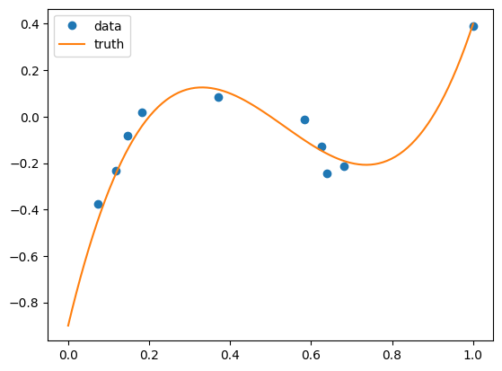
# generate mockup data
n = 10
f = lambda x: 10 * (x - 0.2) * (x - 0.9) * (x - 0.5)

x = np.maximum(np.minimum(rng.normal(0.5, 0.3, n), 1), 0)
y = f(x) + rng.normal(0, 0.05, n)

xx = np.linspace(0, 1, 100)
yy = f(xx)

ax = plt.subplot()
ax.plot(x, y, "o", label="data")
ax.plot(xx, yy, label="truth")
ax.legend()
None
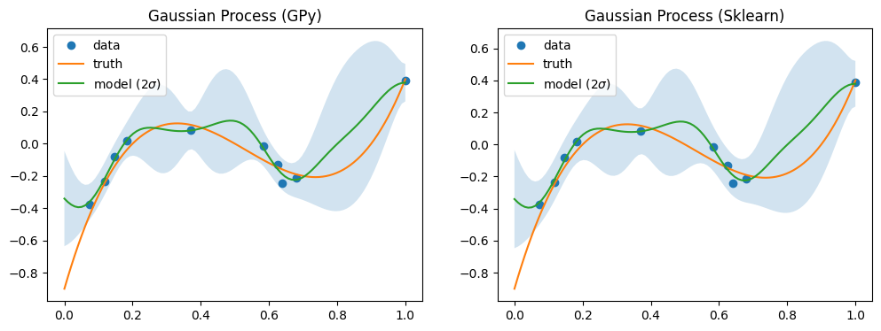
[5]:
# fit two GPs (different implementations)
fig, axs = plt.subplots(1, 2, figsize=(12, 4))
for ax, label in zip(axs, ["GPy", "Sklearn"]):

    sur = Surrogate[label]()
    sur.train(x, y)
    mean, var = sur.predict(xx)

    mean = mean.flatten()
    std = np.sqrt(var.flatten())

    ax.plot(x, y, "o", label="data")
    ax.plot(xx, yy, label="truth")
    ax.fill_between(xx, mean + 2 * std, mean - 2 * std, alpha=0.2)
    ax.plot(xx, mean, label="model ($2 \\sigma$)")
    ax.legend()
    ax.set(title=f"Gaussian Process ({label})")
warning in stationary: failed to import cython module: falling back to numpy
warning in coregionalize: failed to import cython module: falling back to numpy
warning in choleskies: failed to import cython module: falling back to numpy
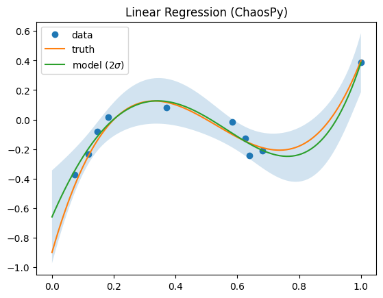
[6]:
# fit with Linear Regression
sur = Surrogate["ChaospyLinReg"](sigma_n=0.1, sigma_p=10, model="monomial", order=5)
sur.train(x, y)
mean, var = sur.predict(xx)

mean = mean.flatten()
std = np.sqrt(var.flatten())

ax = plt.subplot()
ax.plot(x, y, "o", label="data")
ax.plot(xx, yy, label="truth")
ax.fill_between(xx, mean + 2 * std, mean - 2 * std, alpha=0.2)
ax.plot(xx, mean, label="model ($2 \\sigma$)")
ax.legend()
ax.set(title=f"Linear Regression (ChaosPy)")
None
2D
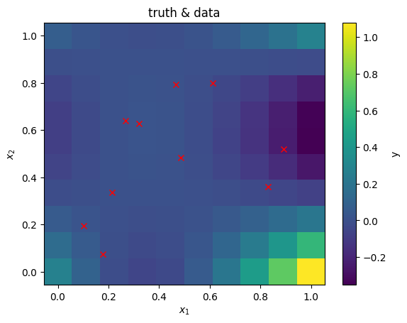
[7]:
# generate mockup data
n = 10
f = lambda x, y: 10 * (x - 0.2) * (y - 0.9) * (x - 0.5) * (y - 0.3)

x = np.maximum(np.minimum(rng.normal(0.5, 0.25, (n, 2)), 1), 0)
y = f(x[:, 0], x[:, 1]) + rng.normal(0, 0.05, n)

xx1 = np.linspace(0, 1, 10)
xx2 = np.linspace(0, 1, 10)
xx1, xx2 = np.meshgrid(xx1, xx2)
xx = np.vstack([xx1.flatten(), xx2.flatten()]).T
yy = f(xx1, xx2)

fig, ax = plt.subplots()
ax.plot(x[:, 0], x[:, 1], "rx")
c = ax.pcolormesh(xx1, xx2, yy, shading="auto")
fig.colorbar(c, label="y")
ax.set(xlabel="$x_1$", ylabel="$x_2$", title="truth & data")
None
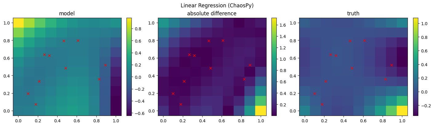
[8]:
# fit with Linear Regression
sur = Surrogate["ChaospyLinReg"](sigma_n=0.1, sigma_p=10, model="hermite", order=4)
sur.train(x, y)
mean, var = sur.predict(xx)

mean = mean.flatten().reshape(xx1.shape)
std = np.sqrt(var.flatten())

fig, axs = plt.subplots(1, 3, figsize=(14, 4), constrained_layout=True)
c = axs[0].pcolormesh(xx1, xx2, mean, shading="auto")
fig.colorbar(c, ax=axs[0])
c = axs[1].pcolormesh(xx1, xx2, np.abs(yy - mean), shading="auto")
fig.colorbar(c, ax=axs[1])
c = axs[2].pcolormesh(xx1, xx2, yy, shading="auto")
fig.colorbar(c, ax=axs[2])
axs[0].set(title=f"model")
axs[1].set(title=f"absolute difference")
axs[2].set(title=f"truth")
for i in range(3):
    axs[i].plot(x[:, 0], x[:, 1], "rx")
fig.suptitle(f"Linear Regression (ChaosPy)")
None